Neural Style Transfer: From-Scratch (VGG-19) vs. Pre-Trained (TF Hub)
Frameworks used: Python, TensorFlow, Keras, Git
Link to Github repo
Introduction
Ars longa, vita brevis. In this project, we apply neural style transfer to transform landscape photos to mimic the artistic styles of Claude Monet and Erin Hanson.
We explore two approaches:
From scratch (Gatys et al., 2015): Build a style transfer loop using VGG-19’s intermediate convolutional layers and TensorFlow ops. This gives full control over losses and optimization.
Pre-trained (Ghiasi et al., 2017): Use TensorFlow Hub’s arbitrary-style model for quick, consistent results with minimal setup.
To clarify inputs in the pipeline:
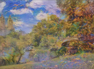
- Content image – the photo to stylize (e.g., Central Park’s Bow Bridge).
- Style image – the artwork whose style you want to emulate (e.g., Monet/Hanson).
- Combination image – the evolving output updated via gradient steps until it blends content + style.
Content examples: Central Park’s Bow Bridge (two views).
Style examples: Erin Hanson’s Layered Light; Monet’s Bridge over a Pond of Water Lilies and Pathway in Garden at Giverny.
Methodology
One key insight from Gatys et al.: instead of updating model weights via gradient descent (as in typical ML), style transfer updates image pixels. We pass the image through early CNN layers to get content and style activations, compute losses, and adjust pixels to minimize a combined loss.
Because pushing the image to better match style can reduce content fidelity (and vice versa), the loss function balances both:
- Content loss compares activations at a deeper layer (e.g., VGG-19 block5 conv2).
- Style loss compares Gram matrices of activations across several earlier layers (captures feature correlations/patterns).
- Total variation loss (TVL) regularizes high-frequency artifacts for smoother outputs.
We use VGG-19 (trained on ImageNet’s 1.2M images, 1,000 classes). It generalizes well to arbitrary photos and produces informative feature maps. For our content image (Figure 1 in the original post), VGG-19’s top-5 predictions—castle, palace, church, monastery, lakeside—align with the scene (San Remo building + lake).
VGG-19 predicted classes (example)
| VGG-19 Object Predicted | Confidence |
|---|---|
| Castle | 28% |
| Palace | 22% |
| Church | 9% |
| Monastery | 5% |
| Lakeside | 4% |
Which layers? Gatys et al. found content is well captured by a deeper layer (e.g., block5 conv2), while style is captured by earlier layers (e.g., first convs from blocks 1–5). We follow that setup.
As intuition, early CNN layers learn edges/corners; deeper layers learn more complex patterns. We compute style by converting activations to Gram matrices (feature correlations) and minimizing MSE vs. the style image’s Gram matrices.
Gram matrix (style features)
(Equation illustration omitted here; see repo for the figure.)
Code snippets
Style/content extractor with Gram matrices
class StyleContentModel(tf.keras.models.Model):
  def __init__(self, style_layers, content_layers):
    super(StyleContentModel, self).__init__()
    self.vgg = vgg_layers(style_layers + content_layers)
    self.style_layers = style_layers
    self.content_layers = content_layers
    self.num_style_layers = len(style_layers)
    self.vgg.trainable = False

  def gram_matrix(self, input_tensor):
    result = tf.linalg.einsum('bijc,bijd->bcd', input_tensor, input_tensor)
    input_shape = tf.shape(input_tensor)
    num_locations = tf.cast(input_shape[1]*input_shape[2], tf.float32)
    return result / (num_locations)

  def call(self, inputs):
    # Expects float input in [0,1]
    inputs = inputs * 255.0
    preprocessed = tf.keras.applications.vgg19.preprocess_input(inputs)
    outputs = self.vgg(preprocessed)
    style_outputs, content_outputs = (outputs[:self.num_style_layers],
                                      outputs[self.num_style_layers:])
    style_outputs = [gram_matrix(s) for s in style_outputs]
    content_dict = {n: v for n, v in zip(self.content_layers, content_outputs)}
    style_dict = {n: v for n, v in zip(self.style_layers, style_outputs)}
    return {'content': content_dict, 'style': style_dict}

extractor = StyleContentModel(style_layers, content_layers)
results = extractor(tf.constant(content_image))
We can then leverage the content and style feature maps returned by calling our extractor object on our input image to compute our style and content losses using the below style_content_loss() function. As can be gleaned in the code, in the case of our style loss we are summing the matrix mean squared errors for each of our five layers’ style and combined image Gram matrices returned by our extractor object, while similarly for our content loss we are performing one mean squared error computation on the single set of activations returned by our extractor for our content and combined images.
def style_content_loss(outputs, content_targets, style_targets, style_weight = 1e-2, content_weight = 1e4):
    style_outputs = outputs['style']
    content_outputs = outputs['content']
    style_loss = tf.add_n([tf.reduce_mean((style_outputs[name]-style_targets[name])**2)
                           for name in style_outputs.keys()])
    print([name for name in style_outputs.keys()])
    style_loss *= style_weight / num_style_layers

    content_loss = tf.add_n([tf.reduce_mean((content_outputs[name]-content_targets[name])**2)
                             for name in content_outputs.keys()])
    print([name for name in content_outputs.keys()])
    content_loss *= content_weight / num_content_layers
    loss = style_loss + content_loss
    return loss

style_targets = extractor(style_image)['style']
content_targets = extractor(content_image)['content']
image = tf.Variable(content_image)
One additional loss component to be added to our total loss function concerns limiting the number of high frequency artifacts produced in our combined image. We can limit these using a standard total variation loss (“TVL”) that acts as a regularization term on the high frequency components of an image:
def high_pass_x_y(image):
  x_var = image[:, :, 1:, :] - image[:, :, :-1, :]
  y_var = image[:, 1:, :, :] - image[:, :-1, :, :]
  return x_var, y_var

def total_variation_loss(image):
  x_deltas, y_deltas = high_pass_x_y(image)
  return tf.reduce_sum(tf.abs(x_deltas)) + tf.reduce_sum(tf.abs(y_deltas))
With this high variation loss function implemented we can then create our gradient descent function using a standard Adam optimizer. This functions computes our style and content losses as well as total variation loss at each step in order to calculate and apply gradient updates to our pixel values using an Adam optimizer:
total_variation_weight=30
opt = tf.optimizers.Adam(learning_rate=0.02, beta_1=0.99, epsilon=1e-1)

@tf.function()
def train_step(image):
  with tf.GradientTape() as tape:
    outputs = extractor(image)
    loss = style_content_loss(outputs)
    loss += total_variation_weight*tf.image.total_variation(image)

  grad = tape.gradient(loss, image)
  opt.apply_gradients([(grad, image)])
  image.assign(clip_0_1(image))
Altogether this stepwise gradient descent process can therefore be summarized as:
- Style Loss: Pass input image to first convolutions of deep layers 1-5 of our VGG-19 model to extract feature maps to calculate style loss
- Compute Gram matrices of style feature maps from (1) and compute matrix mean squared error versus target style image Gram matrix to calculate style loss
- Multiply style loss by style loss weight and add to our total loss
- Content Loss: Pass input image to the second convolution of deep layers 5 of our VGG-19 model to extract feature map to calculate content loss
- Compute matrix mean squared error of feature map resulting from (4) versus original content image to calculate content loss
- Multiply content loss by content loss weight and add to our total loss
- Total Variation Loss: Compute total variation loss of our image by using a standard regularization term on high frequency artifacts in our image
- Multiply TVL by TVL weight and add to our total loss
- Gradient Updates: Calculate gradients of our pixel values in the direction that reduces total loss computed from (8) and update pixel values
- Repeat steps (1) - (9) until convergence
Results
Applying this process using Central Park’s Bow Bridge and Erin Hanson’s Layered Light as our content and style images respectively produces the below output, interactively displaying our pixel gradient updates in real time:


Figure 8. Visualization output of applying gradient descent process to content image pixel values
For our second approach, we simply use a pre-trained neural artistic stylization network originally proposed by Ghiasi et al. and made available through Tensorflow’s model hub in order to visualize differences in their model outputs, producing the below results shown in Figures 9-11.
hub_model = hub.load('https://tfhub.dev/google/magenta/arbitrary-image-stylization-v1-256/2')

for style_image in style_images:
  print('{} style image used'.format(style_image))
  for content_image in content_images:
    content_image_ = load_img(content_image)
    style_image_ = load_img(style_image)
    start_time = time.time()
    stylized_image = hub_model(tf.constant(content_image_), tf.constant(style_image_))[0]
    stylized_image = tensor_to_image(stylized_image)
    display(stylized_image)
Given Ghiasi et al. implement their solution using a different model backbone by training two separate style prediction and style transfer networks on a corpus of 80,000 images, the result of passing our same content and style images to their model is expectedly quite different than from leveraging our bootstrapped model version as can be seen in Figure 9:


Figure 9. Content, style and output images of second neural style transfer approach using Ghiasi et al.’s pre-trained style transfer network


Figure 10. Content, style and output images of second neural style transfer approach using Ghiasi et al.’s pre-trained style transfer network


Figure 11. Content, style and output images of second neural style transfer approach using Ghiasi et al.’s pre-trained style transfer network
Conclusion
In this project we implemented neural style transfer following two distinct approaches of (i) building our algorithm from scratch using Tensorflow’s linear algebra functions and following Gatys et al.’s original approach to neural style transfer using convolutional layers of the VGG-19 network and (ii) using the Tensorflow’s model hub’s pre-trained neural artistic stylization network proposed by Ghiasi et al. in order to compare the differing outputs of both implementations.
Our next steps in our explorations would be to experiment with using different VGG-19 convolutional layers to extract our feature maps as well as to test using the layers of different classification models also trained on ImageNet such as Resnet-50 and EfficientNet-B5.
Thanks for reading!